[1]:
import os,sys
%matplotlib inline
import matplotlib.pylab as plt
import pickle
import numpy as np
plt.rcParams['figure.dpi'] = 100
plt.rcParams['savefig.dpi']=300
plt.rcParams['font.family']='sans serif'
plt.rcParams['font.sans-serif']='Arial'
plt.rcParams['pdf.fonttype']=42
# sys.path.append(os.path.expanduser("~/Projects/Github/PyComplexHeatmap/"))
from PyComplexHeatmap import (
    ClusterMapPlotter,HeatmapAnnotation,anno_simple,anno_scatterplot,anno_lineplot,anno_barplot,
    anno_label,anno_boxplot,anno_img,
)
# plt.rcParams
A quick example
[2]:
#Generate example dataset (random)
df = pd.DataFrame(['AAAA1'] * 5 + ['BBBBB2'] * 5, columns=['AB'])
df['CD'] = ['C'] * 3 + ['D'] * 3 + ['G'] * 4
df['EF'] = ['E'] * 6 + ['F'] * 2 + ['H'] * 2
df['F'] = np.random.normal(0, 1, 10)
df.index = ['sample' + str(i) for i in range(1, df.shape[0] + 1)]
df_box = pd.DataFrame(np.random.randn(10, 4), columns=['Gene' + str(i) for i in range(1, 5)])
df_box.index = ['sample' + str(i) for i in range(1, df_box.shape[0] + 1)]
df_bar = pd.DataFrame(np.random.uniform(0, 10, (10, 2)), columns=['TMB1', 'TMB2'])
df_bar.index = ['sample' + str(i) for i in range(1, df_box.shape[0] + 1)]
df_scatter = pd.DataFrame(np.random.uniform(0, 10, 10), columns=['Scatter'])
df_scatter.index = ['sample' + str(i) for i in range(1, df_box.shape[0] + 1)]
df_heatmap = pd.DataFrame(np.random.randn(30, 10), columns=['sample' + str(i) for i in range(1, 11)])
df_heatmap.index = ["Fea" + str(i) for i in range(1, df_heatmap.shape[0] + 1)]
df_heatmap.iloc[1, 2] = np.nan
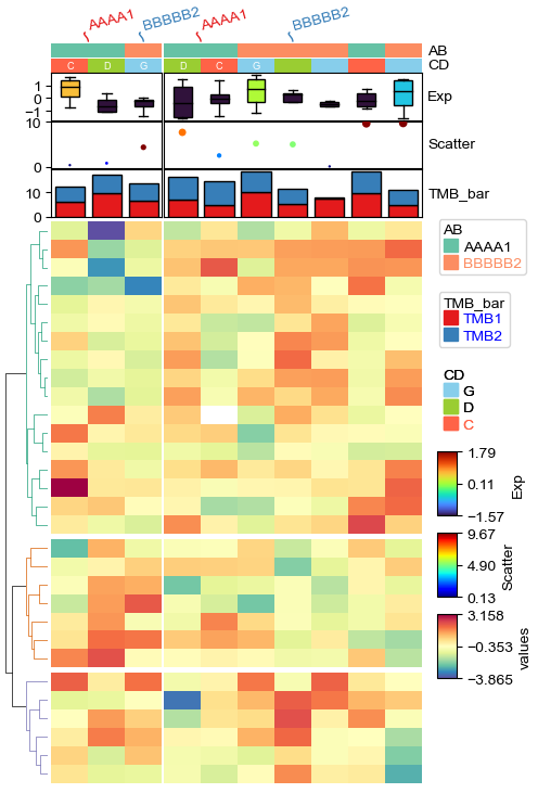
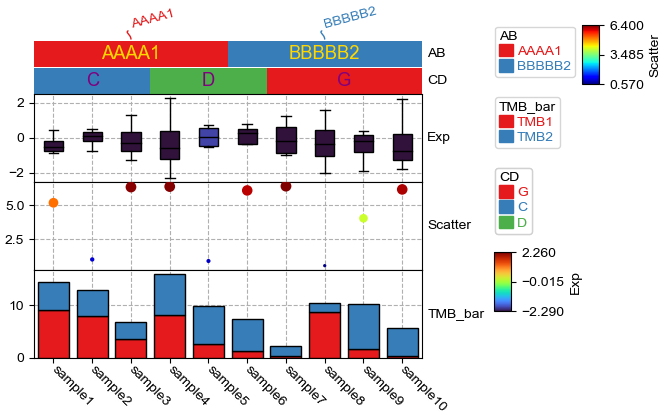
plt.figure(figsize=(4, 6))
col_ha = HeatmapAnnotation(label=anno_label(df.AB, merge=True,rotation=15),
AB=anno_simple(df.AB,cmap='Set2'),axis=1,
CD=anno_simple(df.CD,add_text=True,colors={'C':'tomato','D':'yellowgreen','G':'skyblue'},
legend_kws={'frameon':False}),
Exp=anno_boxplot(df_box, cmap='turbo',height=10),
Scatter=anno_scatterplot(df_scatter,height=10),
TMB_bar=anno_barplot(df_bar,height=10,legend_kws={'color_text':False,'labelcolor':'blue'}),
rasterized=True)
cm = ClusterMapPlotter(data=df_heatmap, top_annotation=col_ha, col_split=2, row_split=3, col_split_gap=0.5,
row_split_gap=1,label='values',row_dendrogram=True,show_rownames=False,show_colnames=False,
tree_kws={'row_cmap': 'Dark2'},cmap='RdYlBu',rasterized=True,
legend_kws=dict(extend='both',extendfrac=0.1,#boundaries=[-2,0,1,2,3],ticks=[-2,0,1,2,3]
),
legend_vgap=5,legend_hpad=2,legend_vpad=5,vmin=-2,vmax=3,center=1) #
#legend_vgap is the vertical gap between two legends, legend_hpad is the horizonal space between legend and heatmap, legend_vpad
# is the verticall space between the first legend and the top of axes (legend_anchor).
# cm.ax_heatmap.set_axis_off()
plt.savefig("test.pdf",bbox_inches='tight',dpi=300)
plt.show()
Starting..
Calculating row orders..
Reordering rows..
Calculating col orders..
Reordering cols..
Plotting matrix..
Plotting HeatmapAnnotations
Collecting legends..
Collecting annotation legends..
Plotting legends..
Estimated legend width: 19.051388888888887 mm
Plotting annotations
Only plot the row/column annotation
[3]:
plt.figure(figsize=(6, 4))
col_ha = HeatmapAnnotation(label=anno_label(df.AB, merge=True,rotation=15),
                            AB=anno_simple(df.AB,add_text=True,legend=True,cmap='Dark2'), axis=1,
                            CD=anno_simple(df.CD, colors={'C': 'red', 'D': 'gray', 'G': 'yellow'},
                                           add_text=True,legend=True),
                            Exp=anno_boxplot(df_box, cmap='turbo',legend=True),
                            Scatter=anno_scatterplot(df_scatter), TMB_bar=anno_barplot(df_bar,legend=True),
                           plot=True,legend=True,legend_vgap=3)
col_ha.show_ticklabels(df.index.tolist())
plt.show()
Plotting HeatmapAnnotations
Collecting annotation legends..
anno_label:
anno_label is used to add a text label to the annotatin, parameter merge control whether to merge the adjacent labels with the same text, if merge != True, then, texts would be draw for each columns. We can also annotate the selected rows/cols using anno_label. In the following example, we also set annot=True to show the float value for each cell,linewidths=0.05,linecolor='orange' can be used to control the line and line color for the boarder between cells.
[4]:
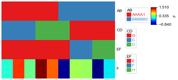
#Annotate the rows with average > 0.3
df_rows = df_heatmap.apply(lambda x:x.name if x.mean() > 0.3 else None,axis=1)
df_rows.name='Selected'

row_ha = HeatmapAnnotation(
            Avg=anno_simple(df_heatmap.mean(axis=1).apply(lambda x:round(x,2)),
                       cmap='jet'), #add_text=True,,text_kws={'rotation':0,'fontsize':10,'color':'black'}
            # Avg=anno_barplot(df_heatmap.mean(axis=1).apply(lambda x:round(x,2)),
            #                height=10,colors='orangered'),
            selected=anno_label(df_rows,colors='red',frac=0.3,rad=0),
            axis=0,verbose=0,label_kws={'rotation':0,'horizontalalignment':'left'})

col_ha = HeatmapAnnotation(
            label=anno_label(df.AB, merge=True,rotation=15),
            AB=anno_simple(df.AB,add_text=True,cmap='Set2'),axis=1,
            Exp=anno_boxplot(df_box, cmap='turbo'),
            verbose=0) #verbose=0 will turn off the log.

plt.figure(figsize=(5.5, 6))
cm = ClusterMapPlotter(
            data=df_heatmap, top_annotation=col_ha,right_annotation=row_ha,
            col_split=2,row_split=2, col_split_gap=0.5,row_split_gap=1,
            label='values',row_dendrogram=True,show_rownames=False,show_colnames=False,
            tree_kws={'row_cmap': 'Set1'},verbose=0,legend_vgap=7,
            #annot=True,linewidths=0.05,linecolor='gold',
            cmap='bwr')
plt.show()
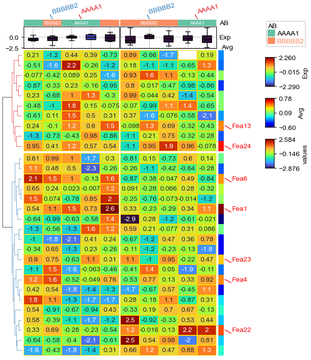
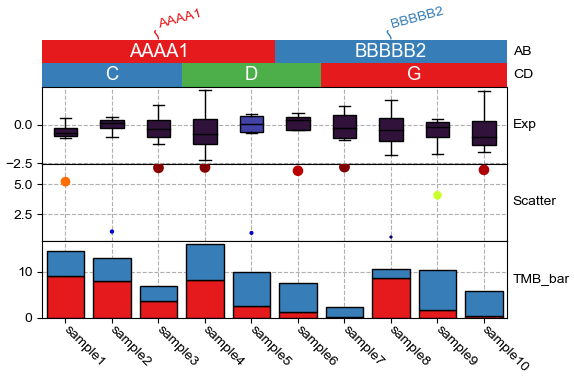
anno_simple:
anno_simple is to draw simple annotatin, cmap for anno_simple can be either categorical (Set1, Dark2, tab10 et.al) or continnuous (jet, turbo, parula). Parameter add_text control whether to add text on the annotation, if the color and fontsize in text_kws was not specified, the color and fontsize would be determined automatically, for example, if the background color is deep, then the text color would be white, otherwise the text color would be black. The text color can be changed with parameter text_kws={‘color’:your_color},for example:
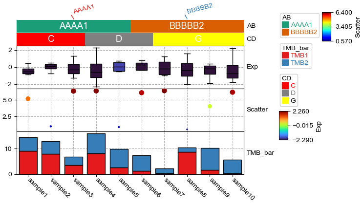
[5]:
plt.figure(figsize=(5, 4))
col_ha = HeatmapAnnotation(label=anno_label(df.AB, merge=True,rotation=15),
                            AB=anno_simple(df.AB,add_text=True,legend=True,text_kws={'color':'gold'}),
                            CD=anno_simple(df.CD,add_text=True,legend=True,text_kws={'color':'purple'}),
                            Exp=anno_boxplot(df_box, cmap='turbo',legend=True),
                            Scatter=anno_scatterplot(df_scatter), TMB_bar=anno_barplot(df_bar,legend=True),
                           plot=True,legend=True,legend_vgap=5,axis=1)
col_ha.show_ticklabels(df.index.tolist())
plt.show()
Plotting HeatmapAnnotations
Collecting annotation legends..
To add a annotation quickly, you just need a dataframe
if df was given, all columns in dataframe df would be treated as a separately anno_simple annotation.
[6]:
plt.figure(figsize=(5, 3))
col_ha = HeatmapAnnotation(df=df,plot=True,legend=True)
plt.show()
Plotting HeatmapAnnotations
Collecting annotation legends..
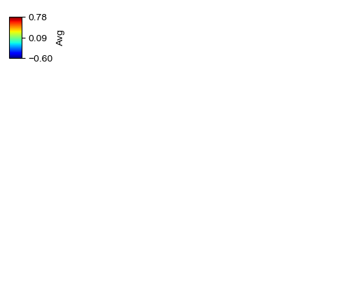
Plot the figure and legend separately
Sometimes, one only want to plot the figure without legend, or plot the legend in a separated pdf, you can do that by giving the parameter plot_legend=False, and plot the legend in another pdf with row_ha.plot_legends
[7]:
plt.figure(figsize=(6, 4))
col_ha = HeatmapAnnotation(label=anno_label(df.AB, merge=True,rotation=15),
                            AB=anno_simple(df.AB,add_text=True,legend=True), axis=1,
                            CD=anno_simple(df.CD,add_text=True,legend=True),
                            Exp=anno_boxplot(df_box, cmap='turbo',legend=True),
                            Scatter=anno_scatterplot(df_scatter), TMB_bar=anno_barplot(df_bar,legend=True),
                           plot=True,legend=True,plot_legend=False,
                           legend_vgap=5,hgap=0)
col_ha.show_ticklabels(df.index.tolist())
plt.show()

plt.figure(figsize=(2,2.5))
row_ha.plot_legends()
plt.show()
Plotting HeatmapAnnotations
No ax was provided, using plt.gca()
Top, bottom, left ,right annotations
[8]:
# Load an example dataset
with open("../data/mammal_array.pkl", 'rb') as f:
    data = pickle.load(f)
df, df_rows, df_cols, col_colors_dict = data
[9]:
df
[9]:
| GSM4412025 | GSM4412026 | GSM4412027 | GSM4412028 | GSM4412029 | GSM4412030 | GSM4412031 | GSM4412032 | GSM4412033 | GSM4412034 | ... | GSM4997945 | GSM4997946 | GSM4997947 | GSM4997948 | GSM4997949 | GSM4997950 | GSM4997951 | GSM4997952 | GSM4997953 | GSM4997954 | |
|---|---|---|---|---|---|---|---|---|---|---|---|---|---|---|---|---|---|---|---|---|---|
| sheep | 1.000000 | 1.000000 | 1.000000 | 1.000000 | 1.000000 | 1.000000 | 1.000000 | 1.000000 | 1.000000 | 1.000000 | ... | 0.435033 | 0.432900 | 0.446626 | 0.449123 | 0.497180 | 0.515918 | 0.483706 | 0.504681 | 0.529076 | 0.446443 |
| beluga whale | 0.687488 | 0.694207 | 0.706525 | 0.702734 | 0.687014 | 0.704003 | 0.705887 | 0.693806 | 0.719417 | 0.712677 | ... | 0.560381 | 0.571552 | 0.610392 | 0.613619 | 0.675832 | 0.668502 | 0.624820 | 0.658377 | 0.702334 | 0.575034 |
| house mouse | 0.000000 | 0.000000 | 0.000000 | 0.000000 | 0.000000 | 0.000000 | 0.000000 | 0.000000 | 0.000000 | 0.000000 | ... | 0.000000 | 0.000000 | 0.000000 | 0.000000 | 0.000000 | 0.000000 | 0.000000 | 0.000000 | 0.000000 | 0.000000 |
| vaquita | 0.693523 | 0.702525 | 0.716792 | 0.725095 | 0.711261 | 0.708651 | 0.717952 | 0.705486 | 0.720915 | 0.724171 | ... | 0.581862 | 0.594443 | 0.628908 | 0.639457 | 0.680801 | 0.707493 | 0.662338 | 0.665142 | 0.751859 | 0.584952 |
| large flying fox | 0.286822 | 0.269406 | 0.296796 | 0.314719 | 0.305074 | 0.308419 | 0.268421 | 0.297236 | 0.295019 | 0.297973 | ... | 0.281684 | 0.363926 | 0.367216 | 0.359392 | 0.289821 | 0.257351 | 0.234301 | 0.295840 | 0.249336 | 0.344848 |
| greater horseshoe bat | 0.530606 | 0.517989 | 0.520719 | 0.525855 | 0.507583 | 0.511993 | 0.528107 | 0.521563 | 0.542159 | 0.509526 | ... | 0.735151 | 0.714805 | 0.708868 | 0.738207 | 0.823604 | 0.828040 | 0.823382 | 0.796882 | 0.878783 | 0.693625 |
| little brown bat | 0.202525 | 0.215990 | 0.238977 | 0.241872 | 0.267750 | 0.236729 | 0.202384 | 0.240519 | 0.251148 | 0.267257 | ... | 1.000000 | 1.000000 | 1.000000 | 1.000000 | 1.000000 | 1.000000 | 1.000000 | 1.000000 | 1.000000 | 1.000000 |
7 rows × 883 columns
[10]:
df_rows
[10]:
| PredictedTaxid | PredictedSpecies | common_names | Family | |
|---|---|---|---|---|
| sheep | 9940.0 | ovis_aries_rambouillet | sheep | Bovidae |
| beluga whale | 9749.0 | delphinapterus_leucas | beluga whale | Monodontidae |
| house mouse | 10090.0 | mus_musculus | house mouse | Muridae |
| vaquita | 42100.0 | phocoena_sinus | vaquita | Phocoenidae |
| large flying fox | 132908.0 | pteropus_vampyrus | large flying fox | Pteropodidae |
| greater horseshoe | NaN | NaN | NaN | NaN |
| bat | 59479.0 | rhinolophus_ferrumequinum | greater horseshoe bat | Rhinolophidae |
| little brown bat | 59463.0 | myotis_lucifugus | little brown bat | Vespertilionidae |
[11]:
df_cols
[11]:
| GSE | Basename | NCBI_scientific_name | taxid | Tissue | Sex | Family | Order | Species | SuccessRate | common_names | |
|---|---|---|---|---|---|---|---|---|---|---|---|
| GSM4412025 | GSE147003 | GSM4412025 | Ovis aries | 9940 | Blood | Female | Bovidae | Artiodactyla | Ovis aries | 0.765818 | sheep |
| GSM4412026 | GSE147003 | GSM4412026 | Ovis aries | 9940 | Blood | Female | Bovidae | Artiodactyla | Ovis aries | 0.797669 | sheep |
| GSM4412027 | GSE147003 | GSM4412027 | Ovis aries | 9940 | Blood | Female | Bovidae | Artiodactyla | Ovis aries | 0.759256 | sheep |
| GSM4412028 | GSE147003 | GSM4412028 | Ovis aries | 9940 | Blood | Male | Bovidae | Artiodactyla | Ovis aries | 0.749813 | sheep |
| GSM4412029 | GSE147003 | GSM4412029 | Ovis aries | 9940 | Blood | Female | Bovidae | Artiodactyla | Ovis aries | 0.770433 | sheep |
| ... | ... | ... | ... | ... | ... | ... | ... | ... | ... | ... | ... |
| GSM4997950 | GSE164127 | GSM4997950 | Eptesicus fuscus | 29078 | Skin | Male | Vespertilionidae | Chiroptera | Eptesicus fuscus | 0.660425 | big brown bat |
| GSM4997951 | GSE164127 | GSM4997951 | Eptesicus fuscus | 29078 | Skin | Male | Vespertilionidae | Chiroptera | Eptesicus fuscus | 0.652822 | big brown bat |
| GSM4997952 | GSE164127 | GSM4997952 | Eptesicus fuscus | 29078 | Skin | Female | Vespertilionidae | Chiroptera | Eptesicus fuscus | 0.664746 | big brown bat |
| GSM4997953 | GSE164127 | GSM4997953 | Eptesicus fuscus | 29078 | Skin | Male | Vespertilionidae | Chiroptera | Eptesicus fuscus | 0.650848 | big brown bat |
| GSM4997954 | GSE164127 | GSM4997954 | Eptesicus fuscus | 29078 | Skin | Male | Vespertilionidae | Chiroptera | Eptesicus fuscus | 0.657170 | big brown bat |
883 rows × 11 columns
[12]:
col_colors_dict
[12]:
{'Tissue': {'#A40043': 'Blood',
  '#00E5FF': 'Brain',
  '#00BECC': 'Cerebellum',
  '#B2F8FF': 'Striatum',
  '#6CBF00': 'Liver',
  '#FFCCEE': 'Muscle',
  '#1E9351': 'Skin'}}
[13]:
#Put annotations on the top
col_ha = HeatmapAnnotation(label=anno_label(df_cols.Family, merge=True, rotation=45),
                               Family=anno_simple(df_cols.Family, legend=True),
                               Tissue=df_cols.Tissue,label_side='right', axis=1)
plt.figure(figsize=(7, 4))
cm = ClusterMapPlotter(data=df, top_annotation=col_ha,
                       show_rownames=True, show_colnames=False,row_names_side='left',
                       col_split=df_cols.Family, cmap='exp1', label='AUC',
                       rasterized=True, legend=True,legend_anchor='ax_heatmap',legend_width=50)
#legend_pad control the space between heatmap and legend.
#plt.savefig("clustermap.pdf", bbox_inches='tight')
plt.show()
Starting..
Calculating row orders..
Reordering rows..
Calculating col orders..
Reordering cols..
Plotting matrix..
Plotting HeatmapAnnotations
Collecting legends..
Collecting annotation legends..
Plotting legends..
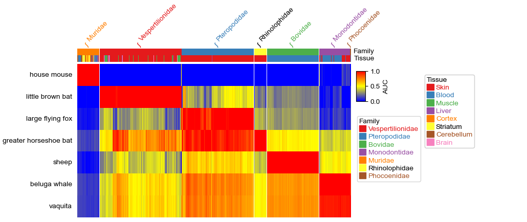
If you have a very long list of legends, the function will automatically increace another column of legend, for example, in the above plot, there are two columns of legends.
[14]:
#Put annotations on the bottom
col_ha = HeatmapAnnotation(Tissue=anno_simple(df_cols.Tissue,height=5),
                           Family=anno_simple(df_cols.Family, legend=False,height=6),
                           label=anno_label(df_cols.Family, merge=True,rotation=-45),
                           label_side='right',axis=1)
plt.figure(figsize=(7, 4))
cm = ClusterMapPlotter(data=df, bottom_annotation=col_ha,
                       show_rownames=True, show_colnames=False,row_names_side='right',
                       col_split=df_cols.Family, cmap='jet', label='AUC',
                       rasterized=True, legend=True)
plt.show()
Starting..
Calculating row orders..
Reordering rows..
Calculating col orders..
Reordering cols..
Plotting matrix..
Plotting HeatmapAnnotations
Collecting legends..
Collecting annotation legends..
Plotting legends..
Estimated legend width: 25.930555555555557 mm
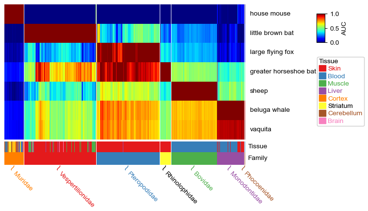
If you want to put the columns annotations on the bottom, then you need to change the order of HeatmapAnnotation, anno_label should be the last one and anno_label(df_cols.Family) should be the second last one. When the columns annotation is on the top, the rotation of the anno_label is 45, but when it is on the bottom, rotation should be -45 (rotate to the other direction). In addition, you can change the row labels to the right by setting row_names_side='right'. It’s
worth noting that the gap betwee the heatmap and the legend could be automatically determined by the code when you set row_names_side to the right. The height of the annotation bar could be changed by the parameter height (mm) in anno_simple or other kinds of annotation functions.
[15]:
#Put annotations on the left
row_ha = HeatmapAnnotation(label=anno_label(df_cols.Family, merge=True,rotation=45),
                           Family=anno_simple(df_cols.Family, legend=True,height=5),
                           Tissue=anno_simple(df_cols.Tissue,height=5),
                           label_side='top',
                           label_kws={'rotation':45,'rotation_mode':'anchor','color':'red'},
                           axis=0)
plt.figure(figsize=(4, 6))
cm = ClusterMapPlotter(data=df.T,left_annotation=row_ha,
                       show_rownames=False, show_colnames=True,col_names_side='top',
                       row_split=df_cols.Family, row_split_gap=0,
                       cmap='exp1', label='AUC',
                       rasterized=True, legend=True,
                       xticklabels_kws={'labelrotation':45,'labelcolor':'blue'},
                       ylabel="Samples",xlabel="Predicted Species",
                       xlabel_kws=dict(labelpad=0),
                       ylabel_kws=dict(labelpad=50),ylabel_bbox_kws=dict(facecolor='green'))
plt.show()
Starting..
Calculating row orders..
Reordering rows..
Calculating col orders..
Reordering cols..
Plotting matrix..
Plotting HeatmapAnnotations
Collecting legends..
Collecting annotation legends..
Plotting legends..
Estimated legend width: 39.68888888888889 mm
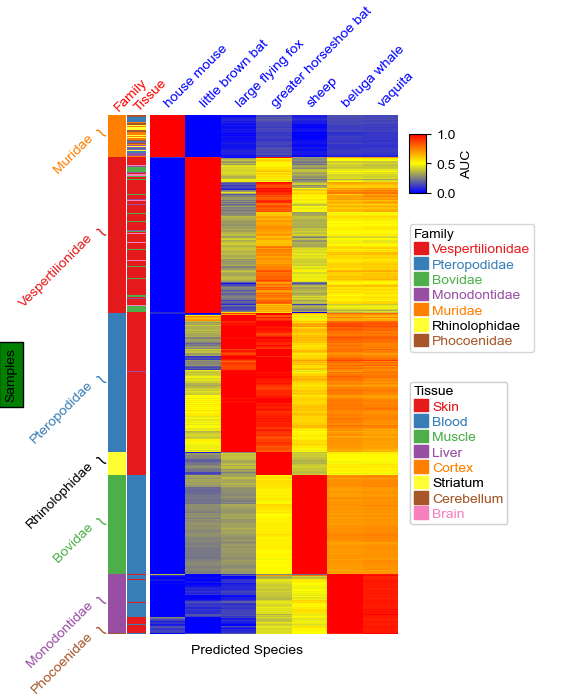
To put annotation on the left in this example, we tranpose the dataframe by useing df.T and use left_annotation. We can put the columns labels on the top by set col_names_side='top' and use xticklabels_kws to change the rotation and color of the columsn labels. We can also change the rotation and color for the annotation labels (for example, Family and Tissue in this plot) by set label_kws={'rotation':45,'rotation_mode':'anchor','color':'red'}.
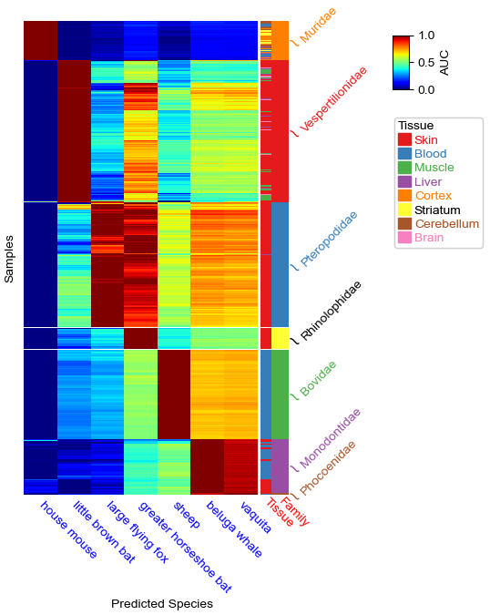
[16]:
#Put annotation on the right
row_ha = HeatmapAnnotation(Tissue=df_cols.Tissue,
                           Family=anno_simple(df_cols.Family, legend=False,height=5),
                           label=anno_label(df_cols.Family, merge=True,rotation=45),
                           label_side='bottom',
                           label_kws={'rotation':-45,'color':'red'},
                           axis=0)
plt.figure(figsize=(4, 6))
cm = ClusterMapPlotter(data=df.T,right_annotation=row_ha,
                       show_rownames=False, show_colnames=True,col_names_side='bottom',
                       row_split=df_cols.Family, cmap='jet', label='AUC',
                       rasterized=True, legend=True,row_split_gap=0.1,
                       xticklabels_kws={'labelrotation':-45,'labelcolor':'blue'},
                       ylabel="Samples",xlabel="Predicted Species")
#plt.savefig("annotation.pdf", bbox_inches='tight')
plt.show()
Starting..
Calculating row orders..
Reordering rows..
Calculating col orders..
Reordering cols..
Plotting matrix..
Plotting HeatmapAnnotations
Collecting legends..
Collecting annotation legends..
Plotting legends..
Estimated legend width: 25.930555555555557 mm