Composite two heatmaps horizontally for mouse DNA methylation array dataset
The dataset used in the following example was obtained from PMID: 36617464
[1]:
import os,sys
%matplotlib inline
# %matplotlib
import matplotlib.pylab as plt
from matplotlib.colors import LinearSegmentedColormap
import pickle
plt.rcParams['figure.dpi'] = 80
plt.rcParams['savefig.dpi']=300
plt.rcParams['font.family']='sans serif'
plt.rcParams['font.sans-serif']='Arial'
plt.rcParams['pdf.fonttype']=42
# sys.path.append(os.path.expanduser("~/Projects/Github/PyComplexHeatmap/"))
import PyComplexHeatmap as pch
pch.use_pch_style()
print(pch.__version__)
1.7.7.dev0+gddb18da.d20240909
[2]:
import pickle
import urllib
f=open("../data/influence_of_snp_on_beta.pickle",'rb')
data=pickle.load(f)
f.close()
beta,snp,df_row,df_col,col_colors_dict,row_colors_dict=data
[3]:
# beta is DNA methylation beta values matrix, df_row and df_col are row and columns annotation respectively, col_colors_dict and row_colors_dict are color for annotation
print(beta.iloc[:,list(range(5))].head(5))
print(df_row.head(5))
print(df_col.head(5))
beta=beta.sample(2000)
snp=snp.loc[beta.index.tolist()]
df_row=df_row.loc[beta.index.tolist()]
                 204875570030_R01C02  204875570030_R04C01  \
cg30848532_TC21             0.525089             0.419515
cg30147375_BC21             0.803776             0.585928
cg46239718_BC21             0.443958             0.517514
cg36100119_BC21             0.351977             0.528846
cg42738582_BC21             0.783958             0.724901

                 204875570030_R05C01  204875570030_R06C01  204875570035_R05C02
cg30848532_TC21             0.483276             0.460750             0.390317
cg30147375_BC21             0.510269             0.831463             0.550146
cg46239718_BC21             0.535909             0.450167             0.564107
cg36100119_BC21             0.524896             0.374422             0.551200
cg42738582_BC21             0.802178             0.848621             0.850481
                   chr  Target  CpG  ExtensionBase ProbeDesign CON  mapFlag  \
cg30848532_TC21  chr12       1    1              0          II   C       16
cg30147375_BC21  chr11       0    0              0          II   C        0
cg46239718_BC21   chr8       1    1              0          II   C        0
cg36100119_BC21  chr19       1    1              0          II   C       16
cg42738582_BC21   chr5       0    0              0          II   C       16

                                        Group  \
cg30848532_TC21      Suboptimal hybridization
cg30147375_BC21                     No Effect
cg46239718_BC21  Artificial low meth. reading
cg36100119_BC21      Suboptimal hybridization
cg42738582_BC21      Suboptimal hybridization

                                                  Type
cg30848532_TC21  1-1-0-CG-GG-II-C-16-GA-chr12-79760438
cg30147375_BC21  0-0-0-ca-ac-II-C-0-AG-chr11-109557651
cg46239718_BC21   1-1-0-cg-gt-II-C-0-GA-chr8-117860829
cg36100119_BC21   1-1-0-CG-GG-II-C-16-GA-chr19-5877949
cg42738582_BC21  0-0-0-AA-AA-II-C-16-AG-chr5-122031379
                       Strain              Tissue     Sex
204875570030_R01C02  MOLF_EiJ  Frontal Lobe Brain  Female
204875570030_R04C01  CAST_EiJ  Frontal Lobe Brain    Male
204875570030_R05C01  CAST_EiJ  Frontal Lobe Brain  Female
204875570030_R06C01  MOLF_EiJ  Frontal Lobe Brain    Male
204875570035_R05C02  CAST_EiJ               Liver    Male
[4]:
row_colors_dict
[4]:
{'Group': {'Artificial high meth. reading': 'darkorange',
  'Artificial low meth. reading': 'skyblue',
  'G-R': 'red',
  'No Effect': 'wheat',
  'R-G': 'green',
  'Suboptimal hybridization': 'darkgray'},
 'Target': {0: 'yellowgreen', 1: 'orangered'}}
[5]:
row_ha = pch.HeatmapAnnotation(
Target=pch.anno_simple(df_row.Target,colors=row_colors_dict['Target'],rasterized=True),
Group=pch.anno_simple(df_row.Group,colors=row_colors_dict['Group'],rasterized=True),
axis=0)
col_ha= pch.HeatmapAnnotation(
label=pch.anno_label(df_col.Strain,merge=True,rotation=15),
Strain=pch.anno_simple(df_col.Strain,add_text=True),
Tissue=df_col.Tissue,Sex=df_col.Sex,
axis=1)
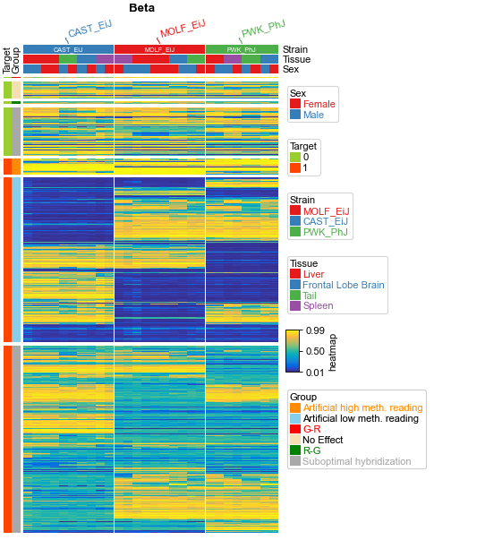
plt.figure(figsize=(5, 8))
cm = pch.ClusterMapPlotter(
data=beta, top_annotation=col_ha, left_annotation=row_ha,
show_rownames=False,show_colnames=False,
row_dendrogram=False,col_dendrogram=False,
row_split=df_row.loc[:, ['Target', 'Group']],
col_split=df_col['Strain'],cmap='parula',
rasterized=True,row_split_gap=1,
legend_anchor='ax_heatmap',legend_vpad=5,
xlabel='Beta',xlabel_side='top',
xlabel_kws=dict(color='black',fontsize=14,labelpad=15),#increace labelpad manually using labelpad (points)
xlabel_bbox_kws=dict(fill=True,edgecolor='blue',boxstyle='round'),
)
# cm.ax.set_title("Beta",y=1.03,fontdict={'fontweight':'bold'})
#plt.savefig("clustermap.pdf", bbox_inches='tight')
plt.show()
Starting..
Calculating row orders..
Reordering rows..
Calculating col orders..
Reordering cols..
Plotting matrix..
Plotting HeatmapAnnotations
Plotting HeatmapAnnotations
Collecting legends..
Collecting annotation legends..
Collecting annotation legends..
Plotting legends..
Estimated legend width: 69.4986111111111 mm
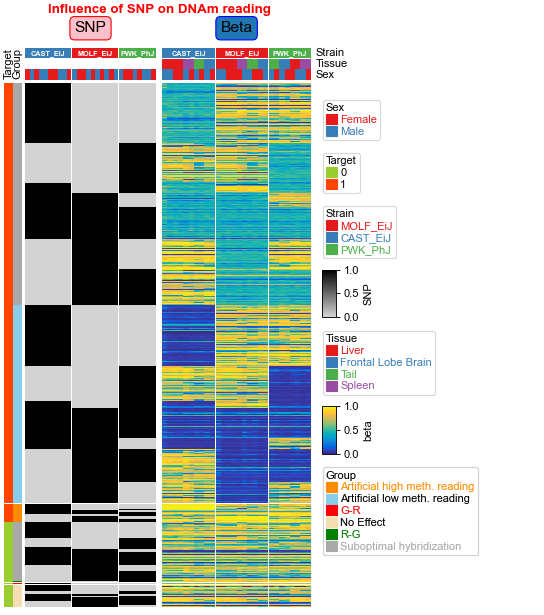
[6]:
row_ha = pch.HeatmapAnnotation(
            Target=pch.anno_simple(df_row.Target, colors=row_colors_dict['Target'], rasterized=True),
            Group=pch.anno_simple(df_row.Group, colors=row_colors_dict['Group'], rasterized=True),
            axis=0)

col_ha1 = pch.HeatmapAnnotation(
            #label=pch.anno_label(df_col.Strain, merge=True, rotation=15),,
            Strain=pch.anno_simple(df_col.Strain, add_text=True,
                              text_kws={'fontweight':'bold'}),
            Tissue=df_col.Tissue, Sex=df_col.Sex,
            axis=1,verbose=0)  # df=df_col.loc[:,['Strain','Tissue','Sex']],

cm1 = pch.ClusterMapPlotter(
            data=beta, top_annotation=col_ha1, left_annotation=None,
            show_rownames=False, show_colnames=False,
            row_dendrogram=False, col_dendrogram=False,
            row_split=df_row.loc[:, ['Target', 'Group']],
            col_split=df_col['Strain'], cmap='parula', #turbo, parula, viridis,
            rasterized=True, row_split_gap=0.1,vmax=1,vmin=0,center=0.5,
            plot=False,label='beta',
            xlabel='Beta',xlabel_side='top',
            xlabel_kws=dict(color='black',fontsize=14,labelpad=10),#increace labelpad manually using labelpad (points)
            xlabel_bbox_kws=dict(fill=True,edgecolor='blue',boxstyle='round')
)

col_ha2 = pch.HeatmapAnnotation(
            #label=pch.anno_label(df_col.Strain, merge=True, rotation=15),,
            Strain=pch.anno_simple(df_col.Strain, add_text=True,
                             text_kws={'fontweight':'bold'}),
            Tissue=df_col.Tissue, Sex=df_col.Sex,
            label_kws={'visible':False},axis=1,verbose=0)

my_cmap = LinearSegmentedColormap.from_list('my_cmap', [(0, 'lightgray'), (1, 'black')])
cm2 = pch.ClusterMapPlotter(
            data=snp, top_annotation=col_ha2, left_annotation=row_ha,
            show_rownames=False, show_colnames=False,
            row_dendrogram=False, col_dendrogram=False,
            col_cluster_method='ward',row_cluster_method='ward',
            col_cluster_metric='jaccard',row_cluster_metric='jaccard',
            row_split=df_row.loc[:, ['Target', 'Group']],
            col_split=df_col['Strain'],
            rasterized=True, row_split_gap=0.1,
            plot=False,legend=True,plot_legend=True,
            cmap=my_cmap,label='SNP',
            xlabel='SNP',xlabel_side='top',
            xlabel_kws=dict(color='black',fontsize=14,labelpad=10),#increace labelpad manually using labelpad (points)
            xlabel_bbox_kws=dict(fill=True,edgecolor='red',boxstyle='round',facecolor='pink')
) # or cmap='gray' or Greys,
cmlist=[cm2,cm1]
[7]:
plt.figure(figsize=(5,8))
ax, legend_axes = pch.composite(cmlist=cmlist, main=0,legend_hpad=2,col_gap=0.1)
# cm1.ax.set_title("title1",y=1.03)
# cm2.ax.set_title("title2",y=1.03)
ax.set_title("Influence of SNP on DNAm reading",y=1.05,fontdict={'fontweight':'bold','color':'red'})
plt.savefig("beta_snp.pdf", bbox_inches='tight')
plt.show()
Starting..
Calculating row orders..
Reordering rows..
Calculating col orders..
Reordering cols..
Plotting matrix..
Plotting HeatmapAnnotations
Collecting legends..
Collecting annotation legends..
Starting..
Calculating col orders..
Reordering cols..
Plotting matrix..
Collecting legends..
Estimated legend width: 69.4986111111111 mm
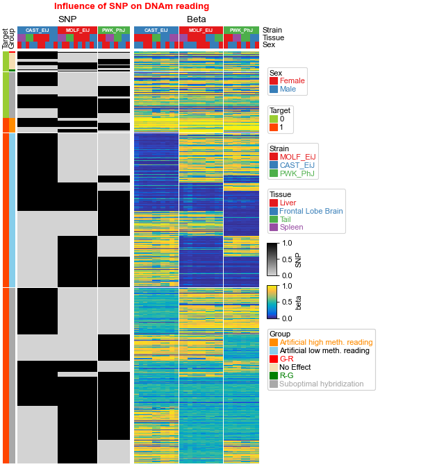
What if the number of column (or row) annotations are different
[8]:
row_ha = pch.HeatmapAnnotation(
            Target=pch.anno_simple(df_row.Target, colors=row_colors_dict['Target'], rasterized=True),
            Group=pch.anno_simple(df_row.Group, colors=row_colors_dict['Group'], rasterized=True),
            axis=0)

col_ha1 = pch.HeatmapAnnotation(
            #label=pch.anno_label(df_col.Strain, merge=True, rotation=15),,
            Strain=pch.anno_simple(df_col.Strain, add_text=True,
                              text_kws={'fontweight':'bold'}),
            Tissue=df_col.Tissue, Sex=df_col.Sex,
            axis=1,verbose=0)  # df=df_col.loc[:,['Strain','Tissue','Sex']],

cm1 = pch.ClusterMapPlotter(
            data=beta, top_annotation=col_ha1, left_annotation=None,
            show_rownames=False, show_colnames=False,
            row_dendrogram=False, col_dendrogram=False,
            row_split=df_row.loc[:, ['Target', 'Group']],
            col_split=df_col['Strain'], cmap='parula', #turbo, parula, viridis,
            rasterized=True, row_split_gap=0.1,vmax=1,vmin=0,center=0.5,
            plot=False,label='beta',
            xlabel='Beta',xlabel_side='top',
            xlabel_kws=dict(color='black',fontsize=14,labelpad=10),#increace labelpad manually using labelpad (points)
            xlabel_bbox_kws=dict(fill=True,edgecolor='blue',boxstyle='round')
)

col_ha2 = pch.HeatmapAnnotation(
            #label=pch.anno_label(df_col.Strain, merge=True, rotation=15),,
            Strain=pch.anno_simple(df_col.Strain, add_text=True,
                             text_kws={'fontweight':'bold'}),
            # Tissue=df_col.Tissue,
            Tissue=pch.anno_spacer(height=3),
            Sex=df_col.Sex,
            label_kws={'visible':False},axis=1,verbose=0)

my_cmap = LinearSegmentedColormap.from_list('my_cmap', [(0, 'lightgray'), (1, 'black')])
cm2 = pch.ClusterMapPlotter(
            data=snp, top_annotation=col_ha2, left_annotation=row_ha,
            show_rownames=False, show_colnames=False,
            row_dendrogram=False, col_dendrogram=False,
            col_cluster_method='ward',row_cluster_method='ward',
            col_cluster_metric='jaccard',row_cluster_metric='jaccard',
            row_split=df_row.loc[:, ['Target', 'Group']],
            col_split=df_col['Strain'],#subplot_gap=5,
            rasterized=True, row_split_gap=0.1,
            plot=False,cmap=my_cmap,label='SNP',
            xlabel='SNP',xlabel_side='top',
            xlabel_kws=dict(color='black',fontsize=14,labelpad=10),#increace labelpad manually using labelpad (points)
            xlabel_bbox_kws=dict(fill=True,edgecolor='red',boxstyle='round',facecolor='pink')
) # or cmap='gray' or Greys,
cmlist=[cm2,cm1]
[9]:
plt.figure(figsize=(5,8))
ax, legend_axes = pch.composite(cmlist=cmlist, main=0,legend_hpad=2,col_gap=0.1)
# cm1.ax.set_title("title1",y=1.03)
# cm2.ax.set_title("title2",y=1.03)
ax.set_title("Influence of SNP on DNAm reading",y=1.05,fontdict={'fontweight':'bold','color':'red'})
# plt.savefig("beta_snp.pdf", bbox_inches='tight')
plt.show()
Starting..
Calculating row orders..
Reordering rows..
Calculating col orders..
Reordering cols..
Plotting matrix..
Plotting HeatmapAnnotations
Collecting legends..
Collecting annotation legends..
Starting..
Calculating col orders..
Reordering cols..
Plotting matrix..
Collecting legends..
Estimated legend width: 69.4986111111111 mm